3 Traditional mediation analysis
Objective of this session
- To learn how to conduct mediation analysis using the traditional approaches.
- Understanding the assumptions and limitations of the methods.
The purpose of mediation analysis is to determine if the effect of a treatment (A) on an outcome (Y) can be explained by a third mediating variable (M). Thus, mediation analysis not only answers whether two variables are related, but also why.
This can be visualized in the following figures.
Overall relationship between A and Y:
Relationship between A and Y through M:
3.1 Traditional approaches for mediation analysis
The two traditional approaches to mediation analysis are the difference method and the product method; also known as the Baron & Kenny-method (1).
The traditional approach use these equations for mediator and outcome (for the case of a continuous mediator and a continuous outcome)
Mediator-model:
\(E(M|A=a, C=c) = \beta_0 + \beta_1a + \beta_2c\) (3.1)
Outcome model with adjustment for mediator:
\(E(Y|A=a, M=m, C=c) = \theta_0 + \theta_1a + \theta_2m + \theta4c\) (3.2)
Outcome model without adjustment for mediator:
\(E(Y|A=a, C=c) = \theta_0' + \theta_1'a + \theta4'c\) (3.3)
Note:
total effect=\(\theta_1'\) , that is the total effect of the independent variable on the dependent variable
direct effect=\(\theta_1\)’, that is the effect of the independent variable on the dependent variable that is not mediated by the mediator
mediation effect=\(\beta1*\theta_2\) (the product method)
mediation effect=’\(\theta_1'-\theta_1\) (the difference method)
Note: The terms ‘mediation effect’ and ‘indirect effect’ are used synonymously.
3.2 An example
In this session, we will use an example to address a mediation research question using both traditional approaches.
It has been suggested that red meat consumption is associated with higher blood glucose levels and an increased risk of Type 2 diabetes (T2D). However, the mechanisms are poorly understood. One hypothesis is that red meat intake affects the level of inflammation, which in turn influence blood glucose.
Does red meat intake directly influence blood glucose levels, or does it act through intermediary mechanisms, such as inflammation? Let’s imagine there exists a hypothetical inflammatory biomarker that serves as a mediator between red meat consumption and blood glucose levels. Therefore, our interest is now how much the effect of red meat on blood glucose is mediated by this inflammatory biomarker. The situation is depicted by below figure.
Does greater consumption of red meat lead to elevated levels of blood glucose by mediating specific inflammation biomarkers?
Example Dataset: A Brief Overview
We’ll explore the relationship between red meat intake and glucose levels in the National Health and Nutrition Examination Survey (NHANES) dataset, which has been modified for this course with simulated variables.
To try this out in practice, we load the NHANES dataset, only keep the variables we need for the example, remove missing data and scale the intake of red meat to be per 65 g/day (i.e., 1-unit higher = 65 g/day).
The variables used in the dataset:
exposure of interest (a): red meat intake (continuous variable, grams per day)
outcome (y): plasma fasting glucose (continuous variable)
mediator (m): a new inflammatory biomarker (continuous variable)
Note that the example is created to demonstrate the methods, and there is no clinical relevance of the results. For the convenience of analysis, we have transformed the mediator (m) and outcome variable (y) so that they follow a normal distribution.
Four demographic variables are considered in the analysis: age, gender, education, and smoking. We assume that adjusting for these four confounding is sufficient to block the backdoor paths. Further discussion on confounding adjustment will be covered in the following session.
3.3 Method 1: Baron & Kenny (the product method)
According to Baron and Kenny (1986) (1), the following criteria need to be satisfied for a variable to be considered a mediator:
- The exposure should be associated with the mediator.
- In the model for the outcome that includes both the exposure and mediator: the mediator should be associated with the outcome.
- In the model for the outcome that includes only the exposure: the exposure should be associated with the outcome.
- When controlling for the mediator, the association between the exposure and outcome should be reduced, with the strongest demonstration of mediation occurring when the path from the exposure to the outcome, when controlling for the mediator is zero.
The following shows the basic steps for mediation analysis suggested by Baron & Kenny.
3.3.1 Step 1: Estimate the relationship between A on M (path a)
That is to check the relation between exposure (red meat) and the mediator (inflammatory biomarker), which corresponds to criteria 1. A mediation makes sense only if A affects M. If A and M have no relationship, M is just a third variable that may or may not be associated with Y.
As the mediator is a continuous variable, we can build a linear regression model, adjusting for confounders on the pathway between A and M.
\((E(M|A=a, C=c)\) = \(\beta_0\) + \(\beta_1a\) + \(\beta_2c\) (3.1)
#>
#> Call:
#> lm(formula = m ~ a + w1 + w2 + w3 + w4, data = nhanes)
#>
#> Residuals:
#>     Min      1Q  Median      3Q     Max
#> -4.2892 -0.6737  0.0135  0.6638  3.9884
#>
#> Coefficients:
#>                       Estimate Std. Error  t value Pr(>|t|)
#> (Intercept)         -1.943e+01  1.339e-01 -145.080   <2e-16 ***
#> a                    2.587e+01  1.493e-01  173.252   <2e-16 ***
#> w1                  -3.177e-04  5.759e-04   -0.552   0.5812
#> w2Male               4.017e-02  2.316e-02    1.734   0.0829 .
#> w3College and above  1.726e-02  2.421e-02    0.713   0.4760
#> w4Yes               -4.038e-02  2.258e-02   -1.789   0.0737 .
#> ---
#> Signif. codes:  0 '***' 0.001 '**' 0.01 '*' 0.05 '.' 0.1 ' ' 1
#>
#> Residual standard error: 1.002 on 8563 degrees of freedom
#> Multiple R-squared:  0.7997, Adjusted R-squared:  0.7995
#> F-statistic:  6836 on 5 and 8563 DF,  p-value: < 2.2e-16
Here, we see that higher red meat intake is positively associated with this new inflammatory biomarker (an increase of 1 unit in red meat consumption is associated with a 25.9 unit increase in the biomarker level).
3.3.2 Step 2: Estimate the relationship between M on Y controlling for A (path b)
That is to build the model between inflammatory biomarker and glucose levels, controlling for red meat intake. This step corresponds to criteria (ii).
\((E(Y|A=a, M=m, C=c) = \theta_0 + \theta_1a + \theta_2m + \theta4c\) (3.2)
#>
#> Call:
#> lm(formula = y ~ a + m + w1 + w2 + w3 + w4, data = nhanes)
#>
#> Residuals:
#>     Min      1Q  Median      3Q     Max
#> -6.9637 -1.3438 -0.0004  1.3949  8.2112
#>
#> Coefficients:
#>                      Estimate Std. Error  t value Pr(>|t|)
#> (Intercept)         17.422689   0.499076   34.910   <2e-16 ***
#> a                   52.686273   0.635020   82.968   <2e-16 ***
#> m                    0.689067   0.021656   31.819   <2e-16 ***
#> w1                   1.500012   0.001154 1299.724   <2e-16 ***
#> w2Male               0.019696   0.046428    0.424    0.671
#> w3College and above  0.014579   0.048520    0.300    0.764
#> w4Yes               -0.025149   0.045252   -0.556    0.578
#> ---
#> Signif. codes:  0 '***' 0.001 '**' 0.01 '*' 0.05 '.' 0.1 ' ' 1
#>
#> Residual standard error: 2.007 on 8562 degrees of freedom
#> Multiple R-squared:  0.9951, Adjusted R-squared:  0.9951
#> F-statistic: 2.889e+05 on 6 and 8562 DF,  p-value: < 2.2e-16
After adjusting for red meat intake, the inflammatory biomarker is associated with higher blood glucose (an increase of 1 unit in the biomarker is associated with 0.69 unit increase in the blood glucose).
3.3.3 Step 3: Estimate the relationship between A on Y (path c)
That is to build the model between red meat intake and glucose levels, without adjusting for the inflammatory biomarker. The only difference between step 2 and step 3 is that mediator is not included in the model.
\((E(Y|A=a, C=c)\) = \(\theta_0'\) + \(\theta_1'a\) + \(\theta4'c\) (3.3)
#>
#> Call:
#> lm(formula = y ~ a + w1 + w2 + w3 + w4, data = nhanes)
#>
#> Residuals:
#>     Min      1Q  Median      3Q     Max
#> -7.3701 -1.4515 -0.0029  1.4438  8.4098
#>
#> Coefficients:
#>                     Estimate Std. Error  t value Pr(>|t|)
#> (Intercept)          4.03412    0.28379   14.215   <2e-16 ***
#> a                   70.50913    0.31635  222.884   <2e-16 ***
#> w1                   1.49979    0.00122 1228.998   <2e-16 ***
#> w2Male               0.04737    0.04908    0.965    0.334
#> w3College and above  0.02647    0.05131    0.516    0.606
#> w4Yes               -0.05298    0.04784   -1.107    0.268
#> ---
#> Signif. codes:  0 '***' 0.001 '**' 0.01 '*' 0.05 '.' 0.1 ' ' 1
#>
#> Residual standard error: 2.122 on 8563 degrees of freedom
#> Multiple R-squared:  0.9945, Adjusted R-squared:  0.9945
#> F-statistic: 3.099e+05 on 5 and 8563 DF,  p-value: < 2.2e-16
We can see that red meat intake is strongly associated with higher glucose levels (an increase of 1 unit in red meat consumption is associated with a 70.5 unit increase in the blood glucose.
Then we can estimate the direct effect and indirect effect:
-
direct effect = \(\theta_1\)
-
indirect effect = \(\beta_1 \theta_2\)
- total effect = \(\theta_1'\)
The direct effect (\(\theta_1\)) of red meat on glucose levels can be assessed by the coefficient of red meat in model b.
The indirect effect can be assessed by calculating the product of \(\beta_1\) \(\theta_2\). In this example, the indirect effect between red meat and glucose levels through inflammatory biomarker is 17.8.
The total effect (\(\theta_1'\)) of red meat on glucose levels can be assessed by the coefficient of red meat in model c, which is 70.5. You might have noticed the total effect also equals the sum of the direct effect and indirect effect.
3.4 Method 2: Difference approach
The difference approach is more commonly used in epidemiology. And the rational of this approach is to compare the effect of A on Y without and with adding M in the models.
If a mediation effect exists, the effect of A on Y will be attenuated when M is included in the regression, indicating the effect of A on Y goes through M. If the effect of A on Y completely disappears, M fully mediates between A and Y (full mediation). If the effect of A on Y still exists, but in a smaller magnitude, M partially mediates between A and Y (partial mediation).
Back to the example, the indirect effect will be the coefficient of red meat in model c (without adjusting for m) minus the coefficient of red meat in model b (adjusting for m), which equals to 17.8.
Note
The algebraic equivalence of the indirect effect using the product method and the difference method will coincide for a continuous outcome on the difference scale (MacKinnon 1995). However, the two methods diverge when using a binary outcome and logistic regression. (MacKinnon and Dwyer 1993).
Note
Recall the four criteria suggested by Baron and Kenny. One of the criteria is that ‘Path C must be significantly different from 0 to ensure there is a total effect between X and Y’. However, this step can be controversial. Even if we don’t find a significant association between X and Y, we could proceed to the next step if we have a strong theoretical basis for their relationship.
Group work - 15 minutes
- Discuss with your group about the two traditional approaches, did you get the same results?
- Discuss the scenarios under which there might be no significant association between A and Y.
3.4.1 Use mediation packages
Now we have estimated the direct and indirect effect using the product and the difference methods.You might have noticed what you got so far are only point estimates, but what if you want to see if this mediation effect is statistically significant (different from zero or not)?
To do so, there are two main approaches: the Sobel test (2) and bootstrapping (3).
Here we will demonstrate that we can use the mediate() function in ‘mediation’ package (4) to conduct mediation analysis. One of the very good options to conduct mediation analysis using the mediation package is we can get confidence interval by bootstrapping.
Let’s load up the R packages.
mediate() takes two model objects as input (\(A \rightarrow M\) and \(A + M \rightarrow Y\)) and we need to specify which variable is an IV (treatment) and a mediator (mediator). For bootstrapping, set boot = TRUE and sims to at least 500.
set.seed(260524)

# Fit mediator model
lm_m <- lm(m ~ a + w1 + w2 + w3 + w4, data = nhanes)
# Fit outcome model
lm_y <- lm(y ~ a + m + w1 + w2 + w3 + w4, data = nhanes)
# Run mediation analysis
results <- mediate(lm_m, lm_y, treat = "a", mediator = "m", boot = TRUE, sims = 10) #can set to 500

summary(results)
#>
#> Causal Mediation Analysis
#>
#> Nonparametric Bootstrap Confidence Intervals with the Percentile Method
#>
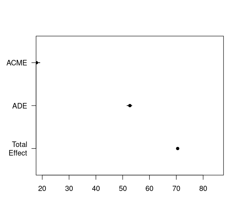
#> Estimate 95% CI Lower 95% CI Upper p-value
#> ACME 17.823 16.906 19.10 <2e-16 ***
#> ADE 52.686 51.612 53.44 <2e-16 ***
#> Total Effect 70.509 70.024 70.85 <2e-16 ***
#> Prop. Mediated 0.253 0.240 0.27 <2e-16 ***
#> ---
#> Signif. codes: 0 '***' 0.001 '**' 0.01 '*' 0.05 '.' 0.1 ' ' 1
#>
#> Sample Size Used: 8569
#>
#>
#> Simulations: 10ADE stands for average direct effects. It describes the direct effect of the A on the Y when controlling for the mediator. Note this estimate is the same as the coefficient We got in the product and difference method. But be aware we are able to get confidence interval and significance levels for the indirect effect, not only its two individual parts by bootstrapping. This is something we need for reporting the mediation.
ACME stands for average causal mediation effects. This is the indirect effect of the IV on the DV that goes through the mediator. Note that ACME estimated to be 17.8, which is the same to the traditional approached we just used.
Total Effect stands for the total effect (direct + indirect) of the IV onto the DV. We can also get it by adding the ACME () and the ADE () to receive the total effect.
Prop. Mediated describes the proportion of the effect of the IV on the DV that goes through the mediator. It’s calculated by dividing the ACME (17.8) by the total effect 70.5) and yields 0.252. The result suggests the mediator (inflammatory biomarker) explains 25.3% proportion of the effect of red meat on glucose levels. We will talk more about proportion mediation in the next session.
For details of the mediate() package, please refer to (4).
3.5 Limitations of the traditional approach
- Non-linearity
- Interactions
- Multiple mediators
3.6 When can we use the traditional approach
When fulfill the criteria, simple tools like regression can be used to estimate a causal mediation effect:
- no unmeasured confounding
- no exposure-mediator interaction
- linear relationship
- rare binary outcome